Data analysis is performed on photoacoustic waveforms by comparing the signals obtained for a sample and a reference compound under the same experimental conditions (temperature, solvent, shape of the beam,...). It is therefore mandatory to leave the laser beam-transducer-cuvette arrangement untouched between sample and reference compounds.
![]()
For evaluation purposes, both for the method of amplitudes and the deconvolution, it is convenient to perform a preprocessing of the experimental data.
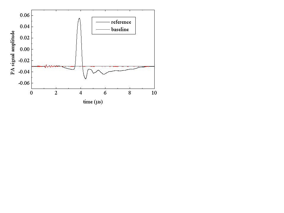
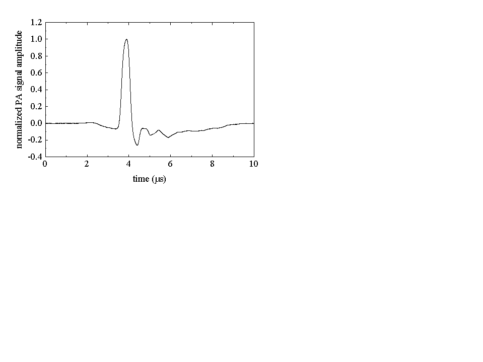
| Photoacoustic signals are generally small, especially when working with aqueous solutions at low temperatures (below 10 °C). This requires high gain amplification (normally x100) and it is common to have small offset in the waveforms, resulting either from the amplifiers or from offsetting the trace on the scope in order to achieve maximum vertical resolution. It is therefore practical to acquire, for each waveform (under the same experimental conditions for both sample and reference compounds), a baseline signal, obtained with no light on the cuvette (by blocking the beam). This baseline is then subtracted and the offsets (common to, say, the reference signal and its baseline) cancel out. In this way the photoacoustic waveforms are net signals oscillating around zero (the picture shows energy, absorbance and amplitude normalized data). Moreover, systematic noise as the noise coming from the laser firing is canceled out in the net waveform. In practice, however, small offest may survive this procedure, and become important when working with the smallest signals. A background correction routine may be of help in the data analysis (vide infra). |
| For several reasons, it is convenient to perform a normalization of
the measured signals vs the laser pulse energy E and the absorbance
of the solution A. For instance this is extermely convenient when
performing deconvolution of experimental waveforms. However, plots
of the measured amplitude Hs vs E or 1-10-A
are traditionally used to improve the data analysis when working with the
method of amplitudes.
Absorbance normalization
Pulse energy normalization
Normalization to the maximum of reference signal
|
![]()
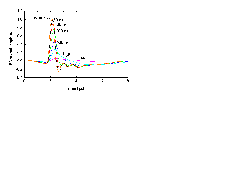
Method of amplitudes
In some special cases of interest, the recovery of thermodynamic information
from the experimentally measured photoacoustic signals can be simply obtained
by using the amplitudes
of the waveforms, neglecting its time dependence.
This simple analysis is possible whenever transient lifetimes are either
much shorter or much longer than the instrumental response of the photoacoustic
setup. As a rule of thumb, this assumption is valid in case:
| short lived transients have lifetimes a factor of 10 below the instrumental response (for a system with a 200 ns risetime, transients with lifetimes below 20 ns are seen as "prompt"); | |
| permanent products or transient species have lifetimes ca 5 times longer than the experimentally determined upper limit of the resolution range (i.e. for a system with a 5 ms upper limit, transients with lifetimes of 25 ms can be considered as "long lived"). |
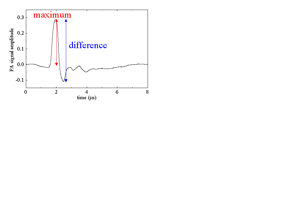
The simplest way is to work with signals from which the baseline has been subtracted. In this case the peak amplitude of the first positive oscillation is a good measure of the photoacoustic signal amplitude. Alternatively, the difference between the amplitudes of the first positive and the first negative oscillations can be considered. The advantage of this second estimate is that it compensates for the presence of residual offsets on the waveforms. When signals are very small and noisy (very dilute samples, very low laser fluences,...) taking the integral of the first positive oscillation may be of help.
Using deconvolution (vide infra) even in the absence of transients with lifetime in the resolution range is an alternative way to reduce the noise and increase accuracy in the recovery of data.
The ratio between the amplitudes of the waveform acquired for the sample under investigation, HSn, and a reference compound, HRn, taken under the same experimental conditions, is then analyzed in terms of the equation (see the phenomenological theory, equation (8)):
Deconvolution
When the lifetimes of the transients under investigation are neither
much longer than the upper limit of the resolution range nor much shorter
than the instrumental response, the method of amplitudes is not practicable
any longer and deconvolution must
be used instead.
The measured signal Hns(t) is a
numerical convolution of the time derivative of the photoinduced, time-dependent
overall volume change (of both structural and enthalpic origin) and the
instrumental response, obtained with a compound releasing all of the absorbed
energy as heat within a few nanoseconds.
The convolution leads to a distorsion of the output Hns(t)
signal both in amplitude an shape. In order to understand the effect
of convolution on the photoacoustic signals, a couple examples are provided,
in which either the preexponential factor or the lifetime is held constant,
whereas the other parameter is varied.
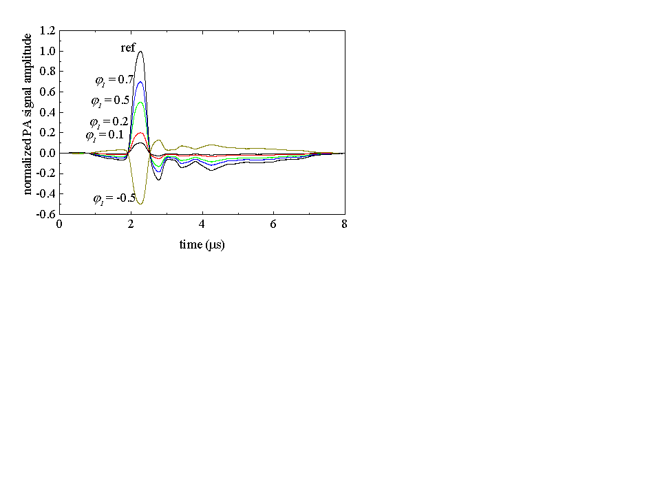
For short lived transients (lifetime below 1
ns), the effect of changing the preeponential factor is simply scaling
the amplitude of the waveform with no change in the time profile.
Negative preexponentials lead to "negative" waveforms, symmetrical with
respect to the time axis.
When the amplitude is kept constant ( in the
example j is kept constant at 1 for all the
waveforms) and the lifetime is changed, both amplitude and shape of the
waveform are affected. When the lifetime increases, the resulting amplitude
becomes smaller and the position of the maximum shifts towards longer times.
The long lived transients (lifetime above 2 ms)
have very small amplitudes (consider that in the example provided the amplitude
was kept at 1) and this hinders the recovery of the kinetic information.
When multiple exponential decays are considered the analysis is generally
perfomed increasing the number of exponentials that are used to fit the
data. The goodness of the fit is judged by the value of the sum of
the squares of the residuals, S2,
and by visual inspection of the residuals and the autocorrelation function
of the residuals. The autocorrelation function of the residuals gives
a good estimate of the randomness of the residuals. Randomly distributed
residuals give autocorrelation functions that are 1 at the first channel
and then drop to approximately 0, oscillating randomly around zero.
The addition of a further exponential function is considered to be reasonable,
if the S2 improves (becomes
smaller) of at least 20 %. The analysis is generally performed using a
least squares optimization based on the Levenberg-Marquardt algorithm.
c2 optimization is not used
in general, since the evaluation of the errors distribution is too time
consuming to be determined for each experiment.
Even for normalized data (divided by E(1-10-A) and
reference scaled to 1) the absolute values of the sum
of residuals S2 depend on
the number of experimental points that are used and the S/N ratio of the
signals. It is therefore not practical to give absolute reference
numbers to judge the goodness of S2.
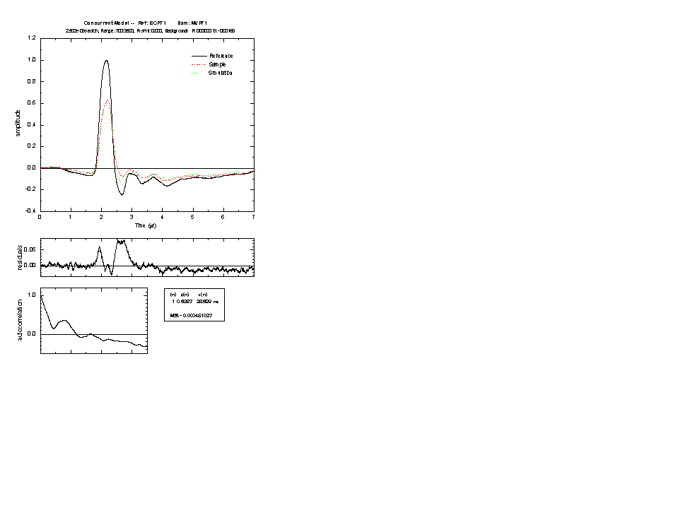
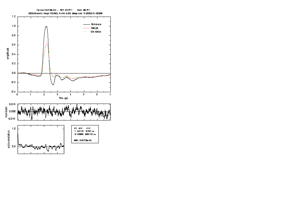
An example is given below, showing signals taken at T = 10 °C for
aqueous solutions of bromcresol purple (reference compound) and o-nitrobenzaldehyde
in the presence of 20 mM of the Major Urinary
Protein (rMUP) at pH 4.5.
Fitting with a single exponential function
results in very correlated residuals. Upon addition of a second
decay, the S2 is reduced
by a factor 20 and the residuals become randomly distributed.
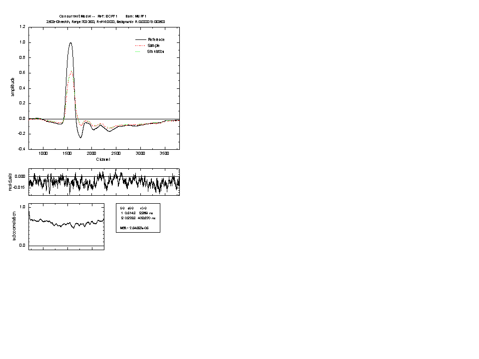
Background search
When background fluctuations are present, the reference and the sample
waveforms may be offset a little bit. An example
is given, for the same data presented above, where an offset has been
added. Although the fit to the sample waveform is reasonable, the
residuals are systematically oscillating below zero, whereas the autocorrelation
functions shows oscillations not around zero, rather around a finite value.
The background search routine allows the optimization
of this offset and eliminates the mismatch between sample and convoluted
waveforms. Great care must be taken in using the background optimization,
especially when long lived (t>2 ms)
transients are under investigation. The addition of an offset may
substantially affect the recovered preexponential factor and lifetime and
may impair the capability of recovering long lived transients.
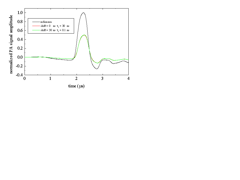
Shift search
Small changes in temperature or small displacement of the laser beam
inside the cuvette (due, for instance, to poiting instability) lead to
small time shifts in the signals. This impairs the capability of
recovering the kinetic parameters from the deconvolution. However,
by time shifting the reference and sample waveforms with respect to each
other, these small variations can be corrected for. Care must be taken
also in optimizing the shift between reference and sample waveforms.
The shifting routine may lead to erroneous evaluations of short (tens of
nanosecond) lifetimes. The presence of a short lived transient (say
30 ns) has effects on the sample waveform which
are very similar to time-shifting the sample with respect to the reference
of an equal amount.
The shift search is important for evaluation of the structural volume
changes in the two-temperatures method.
In this case the shifting is due to the change in the speed of sound between
the two known temperatures. However, even in this case, the shifting
routine must be used with caution in order to avoid systematic errors in
the retrieved parameters. The time shift between reference and sample
waveforms must be carefully evaluated by considering the temperature
dependence of the reference waveform in the solvent used in the experiment.
Special attention must be paid, especially when working with short lived
transients, for which shifting may either mimic or compensate the distorsion
introduced by the relaxation, thus introducing a fake transient or "canceling"
a true one.
![]()
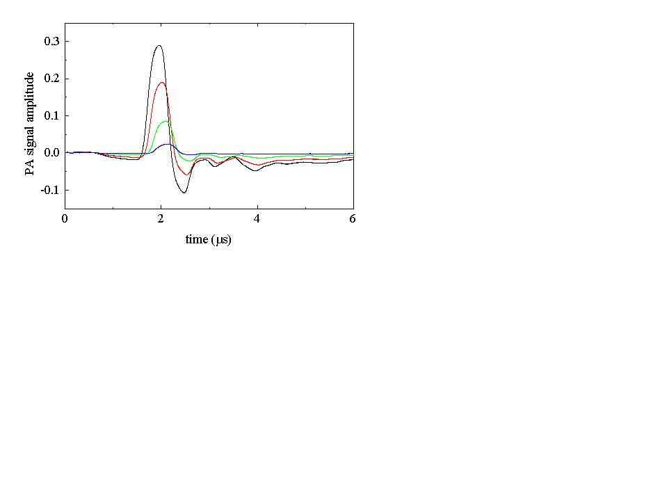
Kinetic schemes
Numerical reconvolution has been performed, so far, assuming multiexponential
relaxation functions.
Even in this case, the answer from a multiexponential fitting can be
interpreted as resulting from a sequential or a parallel scheme.
For the proper interpretation of ji,
it is important to lay down a mechanism. In the case of a sequential reaction
scheme:
![]()
the amplitudes ![]() derived from the reconvolution analysis are
related to the parameters of the elementary steps (i.e., the weight
of each step j i and the
lifetimes ti ) by the following
relations:
derived from the reconvolution analysis are
related to the parameters of the elementary steps (i.e., the weight
of each step j i and the
lifetimes ti ) by the following
relations:
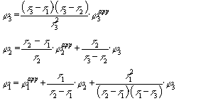
It is obvious that for a system with t3 >> t2 >> t1, the equations simplify and ji = jiapp.
![]()
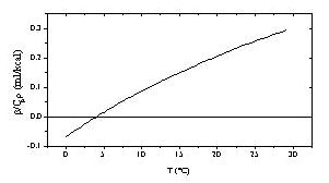
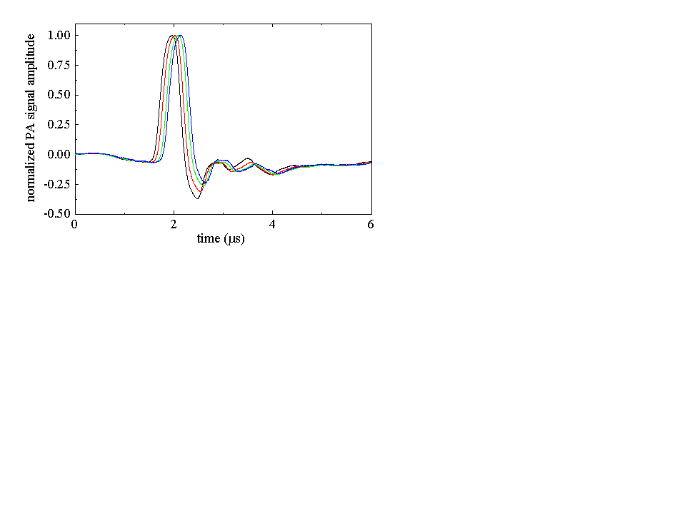
Temperature dependence of photoacoustic signals
The photoacoustic signal of dilute aqueous solutions
depends strongly on the temperature of the solution through
the thermoelastic parameter b/Cpr.
The temperature dependence of b/Cpr
is shown in this figure. As a result, the amplitude
of the photoacoustic signals of an aqueous solution
of bromcresol purple as a function of temperature varies strongly and,
in particular, strongly decreases as the temperature is decreased below
room temperature. In addition, the
speed of sound in the solution depends strongly on the temperature and
therefore the arrival time of the waveform changes as a function of temperature,
resulting in a shift of the waveform when the temperature is changed. This
effect is easily seen for the normalized photoacoustic
signals of an aqueous solution of bromcresol purple as a function of temperature.
In concentrated aqueous solutions of virtually any kind of solute,
this strong temperature dependence is lost and the signal is less affected
by changes in temperature. This is also true for organic solvents.